Tutorial
This tutorial will guide you through your first session using Coquery. You will install a corpus, run a query on that corpus, and visualize the results.
At the end of this tutorial, you will have solved the following task:
- Visualize the occurrences of ten key characters in the twelve chapters of Alice’s Adventures in Wonderland by Lewis Carroll
Starting Coquery
Follow the steps described in download to install Coquery. Once
installed, either choose the Coquery icon from the Applications menu (if you
used the binary installer), or open a terminal, change to the directory
containing the Coquery files, and type ./coquery.py (if you are on
Linux or Mac OS X) or python coquery.py (if you are on Windows).
the main interface will open:
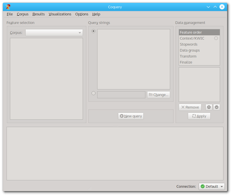
The main interface when launching Coquery for the first time.
Most of the functions in the main interface are inactive. This is so because there is no corpus available yet. We will change this by building our first corpus.
Building the ALICE corpus
The twelve chapters of Alice’s Adventures in Wonderland by Lewis Carroll
(available from Project Gutenberg)
are already provided as text files by Coquery in the the subdirectory
texts/alice of the installation directory. We will use these text files
to build the ALICE corpus.
First, select ‘Corpus manager` from the ‘Corpus’ menu. The corpus manager dialog will open:
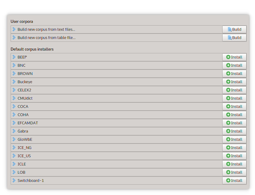
The corpus manager.
Now, click on the green ‘Add’ button  on the entry labelled ‘Build new
corpus...’ to open the Corpus builder:
on the entry labelled ‘Build new
corpus...’ to open the Corpus builder:
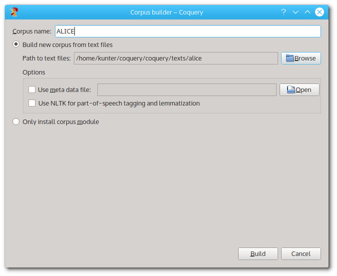
The corpus builder.
The path to the Alice text files is already set up correctly. Type in the name of the new corpus: ALICE, and click on ‘Build’. Leave the other options for later (you can use them later to select a meta file that contains information on each of your corpus files, or to build a corpus with automatic lemmatization and POS tagging, which is provided by the NLTK toolkit).
The corpus builder will take a few moments to load the texts from the file into the new corpus. When finished, you will see an entry ALICE under ‘User corpora’ in the corpus manager. You can click on the entry to see a corpus overview.
When you are finished, close the corpus manager window.
Getting a frequency list
You will notice that now that the ALICE corpus is installed, many more functions in the main interface have become active.
In order to get a frequency list for the words in the ALICE corpus, enter a single asterisk ‘*’ (without quotation marks) into the query string entry field. The asterisk is a wild card that matches any orthographic word in the corpus:
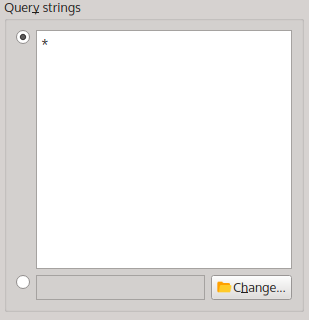
A query string matching any orthographic word.
Next, click on ‘Transformation’ in the data management toolbox in the upper right corner of the main interface. You can choose between different transformations that will be applied to the query results once they are retrieved from the corpus. For example, you can hide all duplicate rows so that only the distinct rows will be shown. In this tutorial, we want to produce a frequency list, so activate the corresponding option:
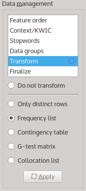
Activating the Frequency list transformation.
Now, it is time to run your first query. Simply click the ‘ New query’
button. After a few moments, a frequency list will be shown in the query
results table:
New query’
button. After a few moments, a frequency list will be shown in the query
results table:
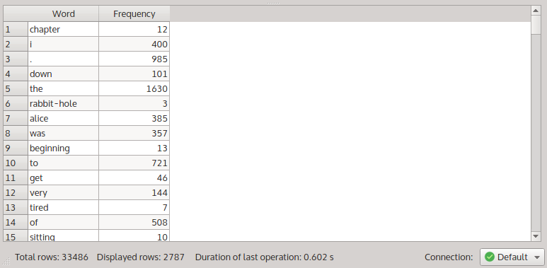
The frequency table from the ALICE corpus.
The status bar informs you that the query matched 33486 tokens. The results table uses the Frequency list transformation, which returns 2787 data rows. This means that the 33486 tokens in the ALICE corpus are split across 2787 different types.
As you can see in the results table, there are 12 tokens of the word chapter, 400 tokens of the word i, 985 tokens of the full stop, and so on.
The current order of types is in the order of appearance in the corpus. You can sort the results table by right-clicking on a table header, and selecting a sorting option from the context menu. If you want to see the most frequent types on top of the results table, select a descending sort order:
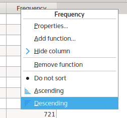
Selecting a descending sorting order for the column Frequency.
The results table will be rearranged instantly. To no great surprise, the comma and the quotation mark are the most frequent types in ALICE, followed by the definite article the, the full stop, and the conjunction and. With a female protagonist, she also ranks relatively high at rank eight. The name Alice appears at rank 14.
You can save the results table by calling ‘Save results’ from the File menu. The table is saved as a file with comma-separated values (CSV). You can use this file in other programs such as OpenOffice/LibreOffice Calc or R/RStudio.
Contingency tables
In the second part of our tutorial task, we want to find out in which chapters from Alice’s Adventures in Wonderland the ten key characters are mentioned.
However, there is a small problem: as your ALICE corpus doesn’t contain any metadata, there is no straightforward way of identifying key characters automatically. We solve this problem by assuming that in a story like Alice’s Adventures, the important characters will be referred to by animate nouns, and that the frequency of the nouns will reflect their importance for the story.
Thus, we go through the sorted word frequency list and find the ten most frequent animate nouns (this excludes, for instance, way, thing, and voice).We enter these nouns as new query strings, each word on a separate line (actually, I cheated and entered the eleven most frequent animate nouns, only because the Cheshire cat was always my favourite character from the book):
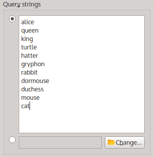
The eleven most frequent animate nouns in ALICE as query strings.
Before we run a new query to get the matches for these query strings, we have to indicate that we also want to include the chapter information in our query result table. We do this by including the corpus feature ‘Filename’ as an additional output column in the results table. We use the ‘Feature selection’ tree in the upper left corner of the main interface for that. Make sure that both ‘Word’ in the ‘Tokens’ table as well as ‘Filename’ in the ‘Files’ table are selected, like in the following picture:
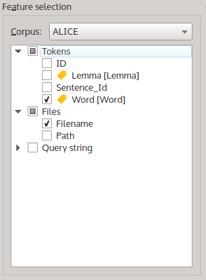
The ‘Feature selection’ tree with ‘Word’ and ‘Filename’ selected.
As you can see in the figure, the checkboxes next to ‘Word’ and ‘Filename’ are ticked. This means that the query will include the information from these two columns in the results table. ‘Word’ was ticked by default, which is why the result table contained the Word column in the first place.
Now, with ‘Word’ and ‘Filename’ selected, click the ‘ New uery’ button to
run a new query. If you followed all steps from the tutorial, your new
results table should look like this:
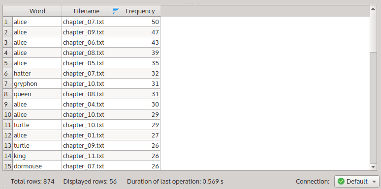
A frequency table for eleven nouns, summarized by ‘Filename’.
Apparently, alice occurs 50 times in chapter 7, 47 times in chapter 9, and so on. You can rearrange these results by switching from the ‘Frequency list’ transformation to ‘Contingency table’. Again, use the data management toolbox for this:

Switching to the ‘Contingency table’ transformation.
You will notice that below the toolbox, the ‘Apply’ button will have become active. Once you click on that button, all pending data management steps will be applied to the results table. You can switch between the different transformations without having to run the query again. This can be very helpful if you are working with corpora that are much bigger than ALICE, as queries can easily take a few minutes or more. For a detailled description of data management in Coquery, see Data management in the Users manual.
For now, press the ‘Apply’ button to produce a contingency table a contingency table instead of the frequency list:
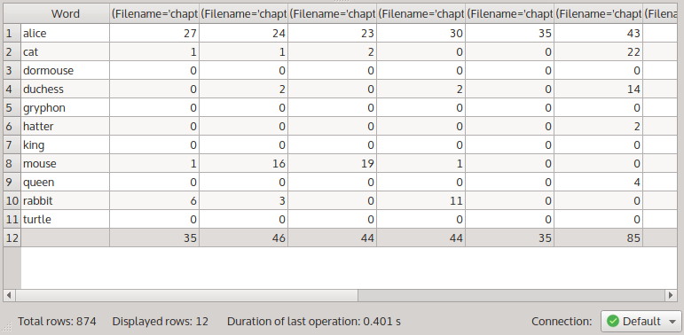
The contingency table for the last query.
In this contingency table, each row corresponds to one noun from the query strings, and each column corresponds to one chapter (use the ‘Feature order’ toolbox if you want to change what appears in the rows and and the columns of a contingency table). We can quickly see for instance that alice is relatively frequent in all chapters, but mouse is mentioned mostly in chapters 2 and 3.
Visualizing the results
The frequency table and the contingency table can already tell us a lot about the distribution of the key characters within the Alice story, but by making use of the visualization capabilities of Coquery, we can learn much more.
The visualization designer helps you to visually understand the structure of your query results. You can open the designer by selecting ‘Visualization designer’ from the ‘Results’ menu:
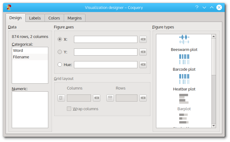
The visualization designer.
The visualization designer consists of three panels: the data selection panel on the left, the figure layout panel in the middle, and the figure selection panel on the right. You can switch between the different tabs which allow you to adjust the labels, the color, and the margins of the figures that you create. This tutorial does not cover these tabs, but you can explore them later.
In order to create a visualization, you first select the columns from the results table that you want to include. In order to do this, you click on one of the columns in the left panel. While keeping the mouse butten pressed, drag the column onto one of the fields in the layout panel. Then, you select a figure type by clicking on one of the icons in the right panel. After a short moment, a figure will be shown.
One particularly useful visualization for analysing token occurrences across a corpus is the ‘Barcode plot’ (users of AntConc will know a similar type of visualization as ‘concordance plots’). We will create a barcode plot that shows in which files the key characters occur.
First, drag the ‘Filename’ column to the field labeled ‘Y’. In this way, the different values of the ‘Filename’ column will be arranged vertically. Next, drag the ‘Word’ column to the field labeled ‘Columns’ under ‘Grid layout’. This is what the visualization designer should look like:
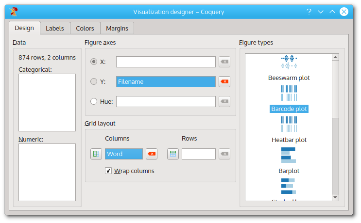
The visualization designer, with ‘Word’ in the ‘Y’ field, and ‘Filename’ in the ‘Column’ field.
Finally, click on the ‘Barcode plot’ icon in the right panel. The following figure will be created:
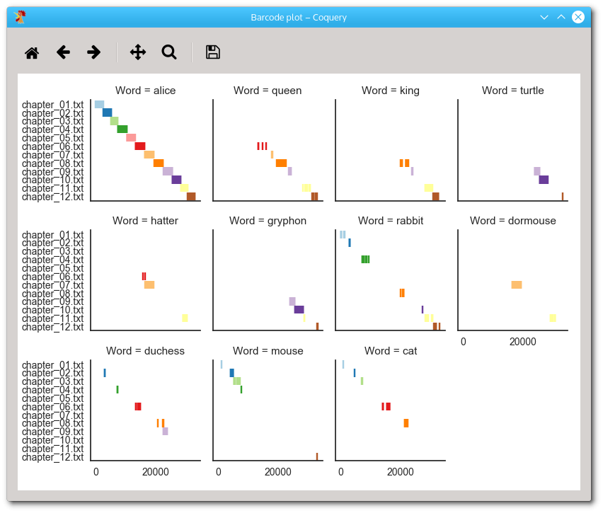
A barcode plot showing the occurrences of each different noun.
As you can see, the plot is actually composed of several subplots, one for each noun in the query string list. Each vertical line in the sub-figures corresponds to one token in the query results table. The horizontal position is the position within the corpus, and the vertical position is the chapter that contains the token. Files are also color-coded so that the same color in different sub-figure corrensponds to the same chapter.
It is easy to see that alice tokens occur frequently in all chapters. Turtle and gryphon tokens occur only in chapters 10 and 11, and no other key character apart from alice occurs in these chapters (apart from with brief appearances of queen, king, and duchess at the beginning of chapter 10). Also co-occurring characters are apparently hatter and dormouse in chapters 6 and 11. It seems as if chapter 11 featured a larger number of key characters than most of the other chapters, but this figure is perhaps not the best visualization to confirm this.
You can easily change the visualization from inside of the designer dialog. Simply drag the ‘Word’ column from the ‘Columns’ field to the ‘Y’ field. This will replace the ‘Filename’ column, which will be returned to the list in the left panel. Drag it to the ‘Columns’ field which was previously occupied by the ‘Word’ column. Now, your visualization designer looks like this:

The visualization designer, with ‘Filename’ in the ‘Y’ field, and ‘Word’ in the ‘Column’ field.
The new barcode plot will look like this:
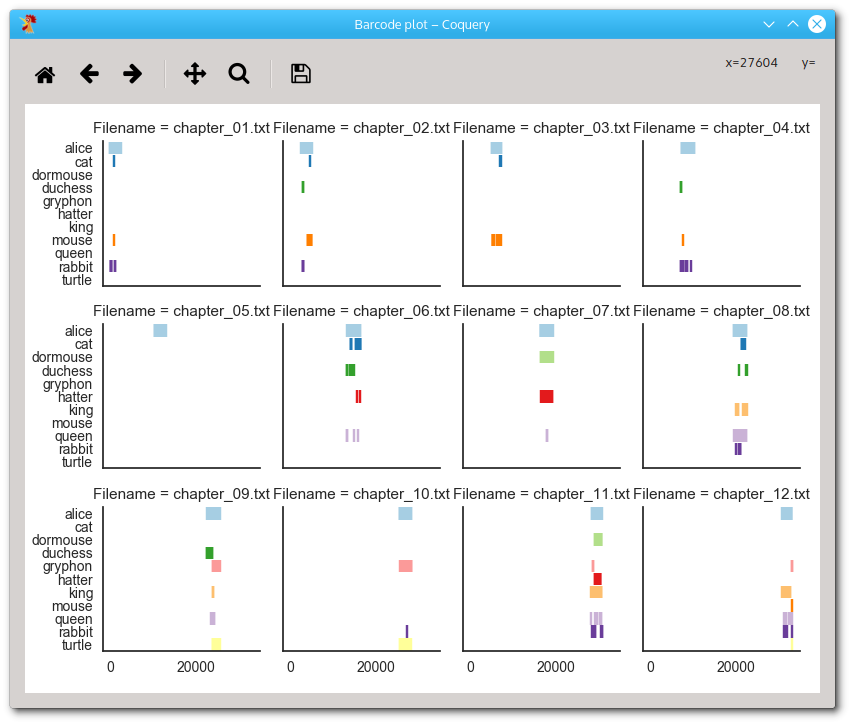
A barcode plot showing the occurrences of key characters in the different chapters.
Indeed, chapter 11 features seven of the eleven key characters (even if gryphon in light-red is mentioned only twice). Conspicuously, the only key character to occur in chapter 5 is alice. The explanation is simple: as the title of chapter 5 Advice from a Caterpillar suggests, we missed at least one key character of the story.
What next?
In this tutorial, you have experimented with a few of the key features of Coquery: specifying query strings, selecting output features, rearranging and transforming the results table, and visualizing the data.
You can learn more about these and other features in the Users manual. A detailed description of the different elements of the main interface and of all menu entries is given in Reference guide. More on building your own corpora, as well as using Coquery with one of the supported third-party corpora, is found in Corpus guide.